
What is Regression? The Problem Setup
Regression is the task of learning a mapping from inputs to a continuous output. Given a training set of \(m\) examples \(\{(\mathbf{x}^{(i)}, y^{(i)})\}_{i=1}^{m}\) where \(\mathbf{x}^{(i)} \in \mathbb{R}^n\) and \(y^{(i)} \in \mathbb{R}\), we want to find a function \(h: \mathbb{R}^n \to \mathbb{R}\) that predicts \(y\) well for new, unseen \(\mathbf{x}\).
The word "regression" (Francis Galton, 1886) originally described a statistical phenomenon — the heights of children "regress toward the mean" compared to their parents. The mathematical machinery he developed became the foundation of modern supervised learning.
The Three Questions Regression Must Answer
- What form should \(h\) take? — We choose a hypothesis class (linear functions, polynomials, etc.).
- What does "predict well" mean? — We choose a loss function to measure prediction error.
- How do we find the best \(h\)? — We choose an optimization algorithm to minimize the loss.
Linear regression gives specific, mathematically justified answers to all three. Crucially, the answers are not arbitrary choices — they fall out of a deep probabilistic assumption about how data is generated. We'll derive this in §06.
In supervised learning, we assume data is drawn i.i.d. from some unknown joint distribution \(P(\mathbf{x}, y)\). We want our hypothesis \(h_{\boldsymbol{\theta}}\) to minimize the expected loss — the population risk. We can only optimize empirical risk (over training data) and hope it generalizes. This tension is the bias-variance tradeoff (§09).
The Linear Model and Hypothesis
Simple Linear Regression (1 Feature)
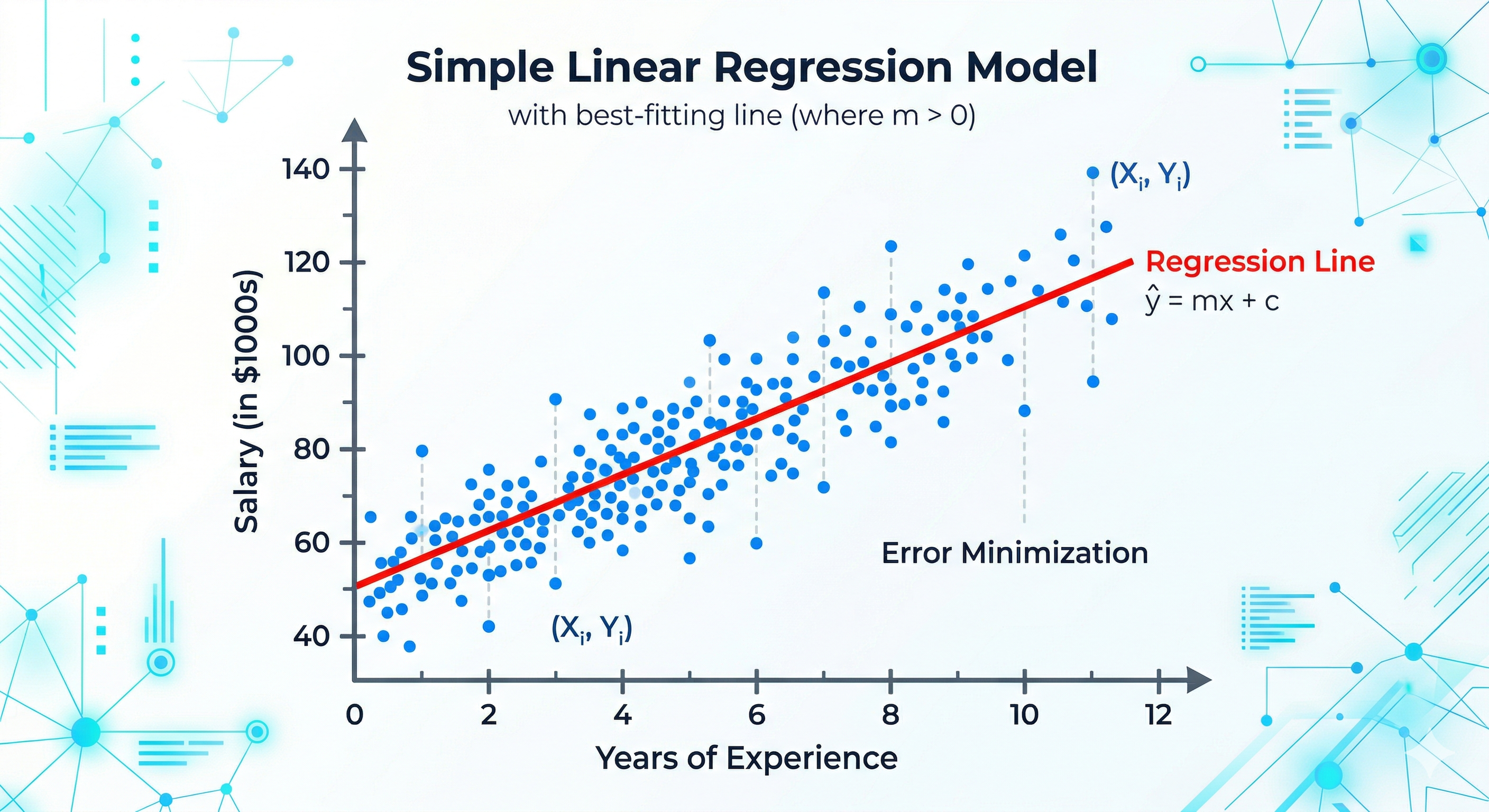
With a single input feature \(x\), the model is a line:
Here \(\theta_0\) is the intercept (the value of \(y\) when \(x = 0\)) and \(\theta_1\) is the slope (the change in \(y\) per unit change in \(x\)). Together they define a line in the 2D plane — we adjust them to fit the data.
Multiple Linear Regression (n Features)
With \(n\) features \(x_1, x_2, \ldots, x_n\):
To simplify notation, we augment the feature vector with a 1: \(\mathbf{x} = [1, x_1, x_2, \ldots, x_n]^T \in \mathbb{R}^{n+1}\) and \(\boldsymbol{\theta} = [\theta_0, \theta_1, \ldots, \theta_n]^T \in \mathbb{R}^{n+1}\). Then:
Matrix Form — Full Dataset
For all \(m\) training examples simultaneously, stack feature vectors row-by-row into the design matrix \(\mathbf{X} \in \mathbb{R}^{m \times (n+1)}\):
\[ \hat{\mathbf{y}} = \mathbf{X}\boldsymbol{\theta} \in \mathbb{R}^m \]
The model assumes \(y\) is linear in the parameters \(\boldsymbol{\theta}\) — not necessarily linear in the raw features. We can include \(x^2, x^3, \log x\) etc. as columns of \(\mathbf{X}\), and the model is still "linear" in the sense that matters for optimization. This is exactly polynomial regression (§11).
The Loss Function — MSE and Why
We need a number that measures how wrong our predictions are. The most natural choice: measure the difference (residual) between the prediction \(\hat{y}^{(i)}\) and the truth \(y^{(i)}\).
Residuals
The residual for example \(i\) is:
Why not just sum the residuals? Positive and negative residuals cancel. Why not sum absolute values? \(|e|\) is not differentiable at zero — inconvenient for calculus. The standard choice: sum of squared residuals.
The Mean Squared Error (MSE) Loss
The \(\frac{1}{2}\) factor is a computational convenience — when we differentiate, the 2 from the power rule and the \(\frac{1}{2}\) cancel neatly, leaving cleaner gradients. It doesn't affect the location of the minimum.
Why Squared Error Specifically?
Three justifications, each from a different perspective:
- Statistical: If noise is Gaussian (\(\epsilon \sim \mathcal{N}(0, \sigma^2)\)), minimizing MSE is equivalent to Maximum Likelihood Estimation. We prove this rigorously in §06 — MSE isn't arbitrary, it falls out of the assumption \(y = \boldsymbol{\theta}^T\mathbf{x} + \epsilon\).
- Mathematical: The square makes \(J\) a smooth, strictly convex quadratic function of \(\boldsymbol{\theta}\). It has a unique global minimum that can be found analytically or reliably by gradient descent. No other common loss shares all three of these properties.
- Geometric: Minimizing \(\sum e_i^2\) is equivalent to finding the orthogonal projection of \(\mathbf{y}\) onto the column space of \(\mathbf{X}\). This gives the solution its elegant geometric interpretation (§05).
MSE penalizes large errors quadratically — a residual of 10 contributes 100× as much as a residual of 1. This means outliers dominate the loss and can severely distort the fitted line. In that case, consider Mean Absolute Error (MAE) — more robust but non-differentiable at 0 — or Huber loss, which is quadratic for small residuals and linear for large ones.
Alternative Loss Functions
| Loss | Formula | Properties | Use When |
|---|---|---|---|
| MSE | \(\frac{1}{m}\sum e_i^2\) | Smooth, convex, differentiable | Gaussian noise assumed; no outliers |
| MAE | \(\frac{1}{m}\sum |e_i|\) | Robust, but not differentiable at 0 | Outliers present; want median regression |
| Huber | MSE if \(|e|<\delta\), else MAE | Best of both worlds | Moderate outliers; need differentiability |
| Log-Cosh | \(\frac{1}{m}\sum\log\cosh(e_i)\) | Smooth approximation to MAE | Outlier-resistant with smooth gradients |
The Normal Equation — Closed-Form Solution
Because MSE is a convex quadratic in \(\boldsymbol{\theta}\), we can find the exact minimum analytically by setting the gradient to zero. This gives the Normal Equation — one of the most important results in all of statistics.
Full Derivation
When is \(\mathbf{X}^T\mathbf{X}\) Invertible?
\(\mathbf{X}^T\mathbf{X}\) is invertible if and only if \(\mathbf{X}\) has full column rank, i.e., the columns of \(\mathbf{X}\) are linearly independent. It fails when:
- Multicollinearity: Two or more features are perfectly correlated (one is a linear combination of others). E.g., including both "temperature in °C" and "temperature in °F" — they're identical up to scaling.
- Too many features: If \(n+1 > m\) (more parameters than samples), \(\mathbf{X}^T\mathbf{X}\) is singular — infinitely many solutions minimize the loss exactly to zero.
- Duplicate features: Same feature column repeated twice.
When \(\mathbf{X}^T\mathbf{X}\) is singular or near-singular, two remedies exist. The Moore-Penrose pseudoinverse \(\mathbf{X}^{\dagger}\) gives the minimum-norm solution analytically. More practically, Ridge regularization adds \(\lambda\mathbf{I}\) to the matrix: \(\hat{\boldsymbol{\theta}}_{\text{ridge}} = (\mathbf{X}^T\mathbf{X} + \lambda\mathbf{I})^{-1}\mathbf{X}^T\mathbf{y}\), which is always invertible for \(\lambda > 0\). This is not just a numerical trick — it has deep statistical meaning (§12).
Geometric Interpretation — Projection
The Normal Equation has a stunning geometric interpretation that reveals why it has to take exactly this form. This is one of the most beautiful results in linear algebra.
The Column Space Perspective
Think of the \(m\) rows of \(\mathbf{X}\) as giving coordinates. The columns of \(\mathbf{X}\) are \(m\)-dimensional vectors. The set of all possible predictions \(\hat{\mathbf{y}} = \mathbf{X}\boldsymbol{\theta}\) as \(\boldsymbol{\theta}\) varies is the column space of \(\mathbf{X}\): a subspace \(\mathcal{C}(\mathbf{X}) \subseteq \mathbb{R}^m\).
Unless \(\mathbf{y}\) happens to lie exactly in \(\mathcal{C}(\mathbf{X})\) (perfect fit), we cannot achieve zero residual. The best we can do: find the point in \(\mathcal{C}(\mathbf{X})\) closest to \(\mathbf{y}\) in Euclidean distance — minimizing \(\|\mathbf{X}\boldsymbol{\theta} - \mathbf{y}\|^2\). This is exactly the orthogonal projection of \(\mathbf{y}\) onto \(\mathcal{C}(\mathbf{X})\).
Why the Residual Must Be Orthogonal to Col(X)
Optimality requires the residual to be orthogonal to every column of
\(\mathbf{X}\):
\(\mathbf{X}^T(\mathbf{y} - \mathbf{X}\hat{\boldsymbol{\theta}}) = \mathbf{0}\).
Expanding this gives \(\mathbf{X}^T\mathbf{X}\hat{\boldsymbol{\theta}} = \mathbf{X}^T\mathbf{y}\) —
precisely the Normal Equations. The geometry and the algebra are the same thing.
Statistical Foundation — MLE Derivation
Why does everyone use squared error? The most rigorous answer comes from probability theory. If we make a specific assumption about how the data is generated, squared error is the only natural choice.
The Probabilistic Data-Generating Model
Assume the true relationship between inputs and outputs is linear, plus independent Gaussian noise:
This means: the output \(y\) is the linear prediction plus a small random measurement/model error, and these errors are independent, zero-mean, and Gaussian. Under this model:
Maximum Likelihood Estimation
MLE: find \(\boldsymbol{\theta}\) that maximizes the probability of observing the training data. The likelihood is:
This derivation reveals a deep truth: choosing a loss function = choosing a noise model. MSE assumes Gaussian noise. MAE assumes Laplace noise. Huber loss assumes a mixture. Every loss function implicitly encodes a statistical assumption about how residuals are distributed. When you use MSE, you're betting the noise is Gaussian.
Gradient Descent for Linear Regression
While the Normal Equation gives an exact answer, gradient descent is essential when \(n\) is large (matrix inversion becomes too costly). From §02's gradient master class, we have:
Component-Wise Derivation
Let's derive the gradient for a single weight \(\theta_j\) from scratch, to make sure every piece is understood:
The Update Rule
for epoch = 1 to num_epochs:
# Forward pass
y_hat = X @ θ # (m,) predictions
residuals = y_hat − y # (m,) errors
# Compute loss (optional, for monitoring)
J = mean(residuals**2) / 2
# Compute gradient
grad = X.T @ residuals / m # (n+1,)
# Update parameters
θ = θ − α * grad
if ‖grad‖ < ε: break # convergence check
Properties of OLS — The Gauss-Markov Theorem
The OLS estimator \(\hat{\boldsymbol{\theta}} = (\mathbf{X}^T\mathbf{X})^{-1}\mathbf{X}^T\mathbf{y}\) has remarkable statistical properties. The Gauss-Markov theorem tells us it's the best we can possibly do within a class of estimators.
Unbiasedness
The OLS estimator is unbiased — in expectation it equals the true \(\boldsymbol{\theta}^*\).
Variance of the OLS Estimator
The diagonal entries are the variances of individual estimates: \(\text{Var}(\hat{\theta}_j) = \sigma^2 [(\mathbf{X}^T\mathbf{X})^{-1}]_{jj}\). Large variance in \(\hat{\theta}_j\) means the estimate of the \(j\)-th coefficient is unreliable — it would change significantly with a different training set.
This formula reveals exactly when estimates are unreliable: when \((\mathbf{X}^T\mathbf{X})^{-1}\) has large entries — i.e., when the matrix is nearly singular due to multicollinearity.
The Gauss-Markov Theorem
Under the OLS assumptions (linearity, exogeneity \(\mathbb{E}[\boldsymbol{\epsilon}|\mathbf{X}]=\mathbf{0}\), homoscedasticity \(\text{Var}(\boldsymbol{\epsilon})=\sigma^2\mathbf{I}\), no multicollinearity), the OLS estimator is the Best Linear Unbiased Estimator (BLUE): among all linear unbiased estimators, it has the minimum variance.
Formally: for any linear unbiased estimator \(\tilde{\boldsymbol{\theta}} = \mathbf{C}\mathbf{y}\) with \(\mathbb{E}[\tilde{\boldsymbol{\theta}}] = \boldsymbol{\theta}^*\), we have:
(positive semidefinite — every diagonal entry of the difference is ≥ 0). OLS is the tightest possible unbiased linear estimate.
Gauss-Markov says OLS is best among linear unbiased estimators. But a biased estimator with much lower variance can have lower total error (lower MSE = bias² + variance). Ridge regression introduces bias deliberately to reduce variance — often beating OLS in test error. This is the bias-variance tradeoff (§09) in action, and explains why regularization can improve upon the "theoretically optimal" OLS.
Bias-Variance Tradeoff
The expected test error of any estimator decomposes into three fundamental components. Understanding this decomposition is central to all of machine learning.
The Bias-Variance Decomposition
For a test point \(\mathbf{x}_0\) with true value \(y_0 = f(\mathbf{x}_0) + \epsilon\):
Derivation
What Each Term Means
| Term | Meaning | Controlled By |
|---|---|---|
| Bias² | How far off the average prediction is from the truth. High bias = underfitting — the model is too simple to capture the true pattern. | Model complexity, hypothesis class. Linear model fitting a cubic truth has high bias. |
| Variance | How much the prediction changes across different training sets. High variance = overfitting — the model learned training noise. | Model complexity, regularization, training size. More parameters → higher variance. |
| Irreducible | Inherent noise in the data — the best any model can achieve. Cannot be reduced by any algorithm. | Data generation process. \(\sigma^2\) of the true noise. |
Feature Scaling and Normalization
Feature scaling is not optional — it directly affects the geometry of the loss landscape and the convergence behavior of gradient descent.
Why Scaling Matters for Gradient Descent
If feature \(x_1 \in [0, 1]\) and feature \(x_2 \in [0, 10000]\), the loss surface is a highly elongated ellipsoid — the loss changes much faster in the \(\theta_2\) direction. Gradient descent in this landscape:
- Takes tiny, inefficient zigzag steps (ravine problem from gradient descent masterclass)
- Requires very different "ideal" learning rates per parameter
- Converges extremely slowly
After scaling all features to similar ranges, the loss surface becomes nearly circular — gradient descent takes direct paths toward the minimum.
Method 1 — Min-Max Scaling (Normalization)
Use when: you know the bounded range and want values in [0, 1]. Sensitive to outliers (the min/max are pulled by extreme values).
Method 2 — Standardization (Z-Score Normalization)
Use when: features may have outliers or unknown bounds. More robust than min-max. The standard choice for most ML workflows.
Always compute \(\mu_j\) and \(\sigma_j\) on the training set only, then apply the same transformation to the validation and test sets. Computing statistics on the full dataset (including test) is data leakage — your model has indirectly seen test data during training.
Does Scaling Affect the Normal Equation?
No — the Normal Equation always produces the exact minimizer regardless of scaling. But in practice, numerically inverting a poorly-conditioned \(\mathbf{X}^T\mathbf{X}\) (due to very different feature scales) introduces floating-point errors. Scaling improves numerical stability. For gradient descent, scaling is essential. For the Normal Equation, it's good practice.
Polynomial Regression — Extending the Model
Linear regression assumes \(y\) is linear in \(\mathbf{x}\). What if the true relationship is curved? Polynomial regression solves this while remaining within the linear regression framework.
Feature Expansion
For a single feature \(x\), add polynomial features up to degree \(d\):
This is still linear regression — linear in the parameters \(\boldsymbol{\theta}\). Every theorem, gradient formula, and the Normal Equation applies unchanged. The only thing that changed is the design matrix \(\mathbf{X}\) now contains polynomial columns:
Overfitting with Polynomial Regression
A degree-\(d\) polynomial has \(d+1\) parameters. With \(d = m-1\), the model can pass through every training point perfectly — but will wildly oscillate between them (Runge's phenomenon). This is extreme overfitting: zero training error, catastrophic test error.
Low degree → underfitting (high bias). High degree → overfitting (high variance). The optimal degree is selected via cross-validation — training on a subset, evaluating on the held-out portion. Alternatively, regularization (§12) allows using high-degree polynomials while penalizing large coefficients, preventing wild oscillation.
Interaction Terms and General Feature Maps
With multiple features, the polynomial expansion includes cross-terms: \(x_1 x_2, x_1^2 x_2, x_1 x_2^2\), etc. For \(n\) features of degree \(d\), the number of features grows as \(\binom{n+d}{d} = O(n^d)\) — exponential in degree. This is the curse of dimensionality. Kernel methods (like SVR with RBF kernel) handle this implicitly via the kernel trick, computing the dot product in high-dimensional feature space without explicitly constructing it.
Regularization — Ridge, Lasso, Elastic Net
Regularization adds a penalty to the loss that discourages large weights — deliberately introducing bias to reduce variance, improving generalization.
Ridge Regression (L2)
Setting \(\nabla J_{\text{Ridge}} = 0\): \(\mathbf{X}^T\mathbf{X}\hat{\boldsymbol{\theta}} + \lambda\hat{\boldsymbol{\theta}} = \mathbf{X}^T\mathbf{y}\), giving \(\hat{\boldsymbol{\theta}}_{\text{ridge}} = (\mathbf{X}^T\mathbf{X} + \lambda\mathbf{I})^{-1}\mathbf{X}^T\mathbf{y}\). The added \(\lambda\mathbf{I}\) ensures the matrix is always invertible — Ridge simultaneously solves multicollinearity and regularizes.
The gradient descent update with Ridge regularization:
The factor \((1-\frac{\alpha\lambda}{m}) < 1\) is "weight decay" — it shrinks \(\boldsymbol{\theta}\) each step before applying the gradient update. Ridge never drives weights exactly to zero.
Bayesian interpretation: Ridge is MAP estimation with a Gaussian prior \(\theta_j \sim \mathcal{N}(0, 1/\lambda)\). The regularization penalty is the negative log of this prior.
Lasso Regression (L1)
Lasso's \(|\theta_j|\) is not differentiable at zero. The gradient uses the subgradient:
Lasso's key property: it drives many weights exactly to zero, performing implicit feature selection. Geometrically, the L1 ball has corners at the coordinate axes — gradient descent paths tend to land exactly at corners, where some \(\theta_j = 0\).
Bayesian interpretation: MAP estimation with a Laplace prior \(\theta_j \sim \text{Laplace}(0, 1/\lambda)\).
Elastic Net (Ridge + Lasso)
Combines L1 sparsity with L2 stability. When features are correlated, Lasso arbitrarily picks one; Elastic Net tends to group correlated features together.
| Method | Penalty | Effect on Weights | Feature Selection | Closed Form? |
|---|---|---|---|---|
| OLS | None | Unconstrained | No | Yes |
| Ridge | \(\lambda\|\boldsymbol{\theta}\|_2^2\) | Shrinks, never zero | No | Yes |
| Lasso | \(\lambda\|\boldsymbol{\theta}\|_1\) | Drives to exactly zero | Yes | No (subgradient) |
| Elastic Net | \(\lambda_1\|\boldsymbol{\theta}\|_1 + \lambda_2\|\boldsymbol{\theta}\|_2^2\) | Sparse + stable | Yes (grouped) | No |
Assumptions and Diagnostics
OLS is only "best" (Gauss-Markov) when its assumptions hold. Violating them doesn't mean the estimates are wrong — but their statistical properties change.
The true relationship is \(y = \boldsymbol{\theta}^T\mathbf{x} + \epsilon\).
Violation: Residual vs fitted plot shows systematic curve. Fix: add polynomial features.
\(\mathbb{E}[\epsilon | \mathbf{X}] = 0\). Noise doesn't systematically push in one direction.
Violation: Biased predictions. Caused by omitting a relevant variable (omitted variable bias).
Constant variance: \(\text{Var}(\epsilon_i) = \sigma^2\) for all \(i\).
Violation (heteroscedasticity): OLS still unbiased but no longer BLUE. Use WLS or robust SE.
Errors \(\epsilon_i\) and \(\epsilon_j\) are uncorrelated for \(i \neq j\).
Violation (autocorrelation): Common in time series. Use GLS or include lagged features.
\(\mathbf{X}^T\mathbf{X}\) is invertible — no feature is a linear combo of others.
Violation: Coefficients blow up, are unstable. Use Ridge regularization or VIF analysis.
\(\epsilon \sim \mathcal{N}(0,\sigma^2)\). Required for hypothesis tests and confidence intervals.
Violation: OLS still consistent. But t-tests and F-tests are invalid. Use robust inference.
Plot residuals \(e_i\) vs fitted values \(\hat{y}_i\). In a well-specified model: residuals should be randomly scattered around zero with no pattern. A U-shape → nonlinearity (add polynomial features). Funnel shape → heteroscedasticity. Systematic structure → omitted variable. QQ-plot of residuals tests normality.
Evaluation Metrics
| Metric | Formula | Range | Interpretation |
|---|---|---|---|
| MSE | \(\frac{1}{m}\sum(y_i - \hat{y}_i)^2\) | \([0, \infty)\) | Mean squared error. Same units as \(y^2\). Penalizes outliers heavily. |
| RMSE | \(\sqrt{\text{MSE}}\) | \([0, \infty)\) | Same units as \(y\) — interpretable as "average error magnitude". |
| MAE | \(\frac{1}{m}\sum|y_i - \hat{y}_i|\) | \([0, \infty)\) | More robust to outliers. Always \(\leq\) RMSE. |
| R² | \(1 - \frac{\text{SS}_{\text{res}}}{\text{SS}_{\text{tot}}}\) | \((-\infty, 1]\) | Fraction of variance explained. R² = 1: perfect. R² = 0: as good as predicting the mean. Negative: worse than the mean. |
| Adjusted R² | \(1 - (1-R^2)\frac{m-1}{m-n-1}\) | \((-\infty, 1]\) | Penalizes adding useless features. R² always increases with more features; adjusted R² can decrease. |
| MAPE | \(\frac{100}{m}\sum\frac{|y_i-\hat{y}_i|}{|y_i|}\) | \([0, \infty)\%\) | Relative error in %. Useful when scale varies across data. |
R² — Deep Dive
For OLS: \(\text{SS}_{\text{tot}} = \text{SS}_{\text{reg}} + \text{SS}_{\text{res}}\) (total variance = explained + unexplained). So \(R^2 = \frac{\text{SS}_{\text{reg}}}{\text{SS}_{\text{tot}}}\) — the fraction of total variance that the model explains.
R² increases monotonically as you add features, even useless ones — never use it to compare models with different numbers of features. Use adjusted R² or information criteria (AIC/BIC) instead. Also, a high R² does not mean the model is well-specified — it can be high even when assumptions are violated.
Normal Equation vs Gradient Descent
| Normal Equation | Gradient Descent | |
|---|---|---|
| Formula | \((\mathbf{X}^T\mathbf{X})^{-1}\mathbf{X}^T\mathbf{y}\) | \(\boldsymbol{\theta} \leftarrow \boldsymbol{\theta} - \frac{\alpha}{m}\mathbf{X}^T(\hat{\mathbf{y}}-\mathbf{y})\) |
| Solution quality | Exact global optimum | Approximate — converges to optimum |
| Computational cost | \(O(n^3)\) for matrix inversion | \(O(kn)\) total, \(k\) = iterations |
| Works for large \(n\)? | No: \(n > 10^4\) becomes slow/infeasible | Yes: scales to billions of parameters |
| Learning rate? | None needed | Must be chosen carefully |
| Feature scaling? | Not needed for correctness | Essential for fast convergence |
| Non-linear models? | No — only for linear regression | Yes — works for any differentiable loss |
| Multicollinearity? | Fails (singular matrix) | Converges slowly, but still works |
| Regularization | Ridge has closed form: \((\mathbf{X}^T\mathbf{X}+\lambda\mathbf{I})^{-1}\mathbf{X}^T\mathbf{y}\) | Add \(\frac{\lambda}{m}\boldsymbol{\theta}\) to gradient |
Use the Normal Equation when: \(n \leq 10^4\) features and you have a GPU or fast linear algebra library. Use Gradient Descent when: large \(n\), online/streaming data, or for any model beyond linear regression (logistic, neural networks). For your house price prediction project — small \(n\) — the Normal Equation gives the exact answer instantly. For training your ViT chest X-ray classifier — billions of parameters — gradient descent (Adam) is the only option.
The Full Mental Model — Everything Together
The unified story, told once more in plain language:
- Model: Assume \(y = \boldsymbol{\theta}^T\mathbf{x} + \epsilon\) — the world is approximately linear in the features. Represent all \(m\) examples at once with the design matrix \(\mathbf{X}\).
- Loss — MLE tells us: If \(\epsilon \sim \mathcal{N}(0,\sigma^2)\), Maximum Likelihood Estimation is exactly equivalent to minimizing MSE. The loss function is not a heuristic — it encodes a probabilistic assumption about the noise.
- Geometry: Minimizing MSE = finding the orthogonal projection of \(\mathbf{y}\) onto the column space of \(\mathbf{X}\). The residual is orthogonal to every predictor — this is the Normal Equation.
- Closed-form solution: \(\hat{\boldsymbol{\theta}} = (\mathbf{X}^T\mathbf{X})^{-1}\mathbf{X}^T\mathbf{y}\) — exact, in one shot. Costs \(O(n^3)\).
- Iterative solution: \(\boldsymbol{\theta} \leftarrow \boldsymbol{\theta} - \frac{\alpha}{m}\mathbf{X}^T(\hat{\mathbf{y}}-\mathbf{y})\) — scales to any \(n\), required for all nonlinear models.
- Statistical properties: OLS is BLUE (Gauss-Markov). Unbiased with variance \(\sigma^2(\mathbf{X}^T\mathbf{X})^{-1}\). Multicollinearity inflates this variance.
- Regularization: Ridge (L2) shrinks weights, improves conditioning, has closed form. Lasso (L1) drives weights to zero — implicit feature selection. Both trade bias for variance — often improving test error over unregularized OLS.
- Extensions: Polynomial features make the model nonlinear in \(\mathbf{x}\) while keeping it linear in \(\boldsymbol{\theta}\) — the entire framework applies unchanged. Everything in logistic regression (sigmoid, cross-entropy) builds directly on this linear foundation.
Linear regression is not a standalone algorithm — it is the atom from which the rest of ML is built. Logistic regression replaces the identity output with a sigmoid; neural networks stack many linear layers with nonlinear activations; SVMs find the linear separator with maximum margin; PCA finds the linear subspace of maximum variance. Every model you ever trained — contains linear regression at its core. The design matrix, the gradient \(\mathbf{X}^T(\hat{\mathbf{y}}-\mathbf{y})\), the bias-variance tradeoff: these recur everywhere.